In Part 1 of this series, we explored the fundamentals of Amazon Redshift optimization — things like distribution and sort keys, compression encoding, and keeping statistics fresh.
Those alone can deliver 30–60% faster queries in most environments.
But those optimizations are well-known. If you want to get Redshift running at peak efficiency — especially for large, mixed workloads — you need to go deeper.
In this post, we’ll cover advanced tuning techniques and lesser-known AWS analytics features that are often overlooked but can deliver massive improvements in both speed and cost-efficiency.
1. Workload Management (WLM) – Master Your Queues
If you’ve ever had a dashboard grind to a halt during heavy ETL, you’ve seen the impact of poor workload isolation.
By default, Redshift dumps all queries into the same execution pool, letting heavy jobs starve lighter, latency-sensitive queries.
The fix: create separate queues for different workloads using Workload Management.
- Static WLM: Predictable, fixed queue sizes, but needs manual tuning.
- Auto WLM: Dynamic, automatically adjusts resources, better for unpredictable workloads.
Example:
SET query_group TO 'etl';
This routes ETL jobs to a dedicated queue, leaving BI queries unaffected.
Pro tip: Use STL_WLM_QUERY to monitor queue wait times. If you see spikes, that’s your signal to adjust WLM settings.
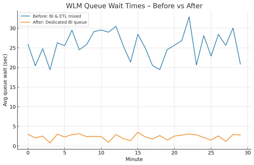
Before: BI queries waited ~25 seconds.
After: Wait dropped to under 2 seconds.
2. Concurrency Scaling – Burst Without Breaking
Even with perfect WLM queues, you can still run into hardware limits during peak load. Concurrency Scaling solves this by spinning up additional capacity automatically.
- First 1 hour/day per cluster is free.
- Best for BI/reporting queues where traffic is unpredictable.
Enable it in WLM settings and apply it only to queues that benefit from burst capacity.
Query times dropped from 18s to ~6s during peak hours.

3. Short Query Acceleration (SQA) – Keep Small Queries Snappy
Small, fast queries — like API lookups or dashboard drilldowns — often get stuck behind long analytical jobs.
With SQA, Redshift identifies and prioritizes them in dedicated slots, bypassing the queue entirely.
Why it’s overlooked: It doesn’t help big queries. It’s all about making small queries consistently instant.
Enable it in WLM with a threshold (default: 1s). For dashboards, this can be the difference between “feels instant” and “feels broken”.
4. Controlled Data Skew – When Uneven is Better
We’re taught to keep data distribution even — but sometimes skew can improve performance.
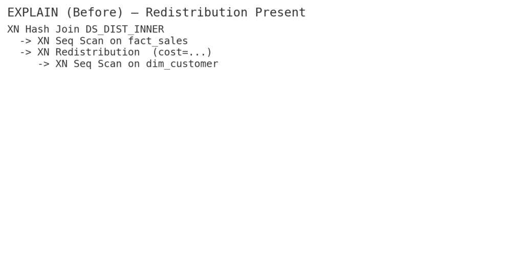
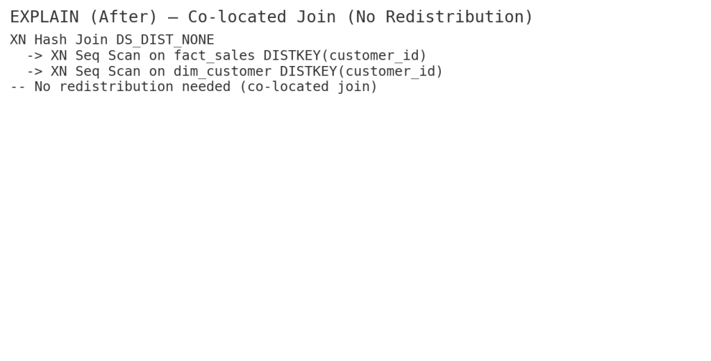
If most queries join on customer_id, using it as the DISTKEY ensures co-located joins, eliminating expensive data redistributions, even if it creates mild skew.
Check skew:
SELECT "table", skew_sortkey1, skew_rows
FROM SVV_TABLE_INFO
WHERE skew_rows > 1.5;
5. Vacuum & Analyze – Smarter, Not Harder
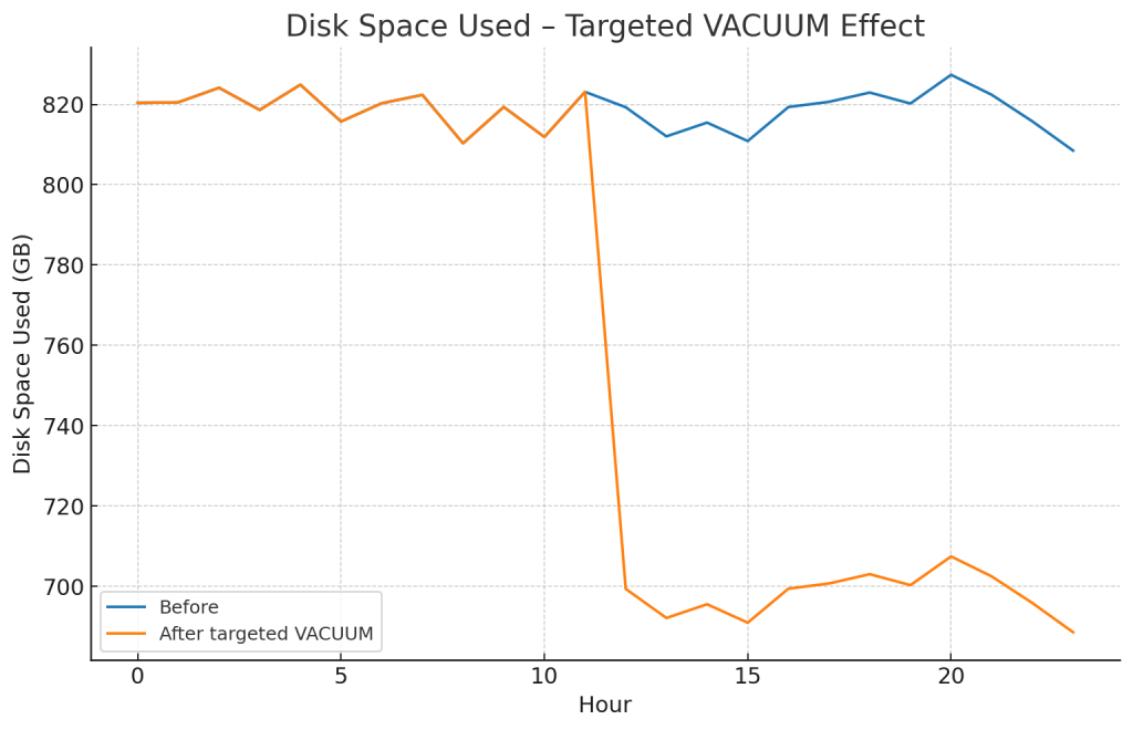
VACUUM and ANALYZE are essential for reclaiming space and keeping stats up-to-date, but running them across the board wastes time and resources.
Instead:
VACUUM my_table TO 80 PERCENT;
ANALYZE PREDICATE COLUMNS my_table;
This reclaims space only if fragmentation is >20% and updates stats only for columns in WHERE clauses.
6. Query-Level Tuning – SQL Still Matters
Sometimes your bottleneck is the query, not the cluster. For example, switching from CTEs to temp tables for repeated aggregations can slash execution time.

- CTE: 9.6s
- Temp Table: 3.2s
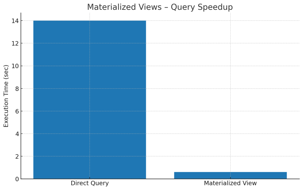
7. Materialized Views – Precompute the Pain
Materialized views store precomputed results for expensive queries. They refresh on demand and can turn a multi-second dashboard load into milliseconds.
Example:
CREATE MATERIALIZED VIEW mv_sales AS
SELECT date, SUM(amount) total_sales
FROM fact_sales
GROUP BY date;
8. Result Caching – Free Performance Boost
If you run the same query multiple times and the underlying data hasn’t changed, enable:
SET enable_result_cache_for_session = ON;
The first run hits storage; subsequent runs return instantly.
Pro tip: Combine with ETL-completion triggers to invalidate cache at the right time.
9. Spectrum Optimization – Query Less, Pay Less
When using Redshift Spectrum for external data:
- Store in Parquet/ORC for efficient scans.
- Partition by high-selectivity columns.
- Filter early for predicate pushdown.
📊 Scan size cut by 87% after optimization:

10. Automatic Table Optimization (ATO) – Let Redshift Adapt
Instead of guessing sort/dist keys, let Redshift decide:
ALTER TABLE my_table ALTER DISTSTYLE AUTO;
ALTER TABLE my_table ALTER SORTKEY AUTO;
ATO adjusts keys based on actual workload patterns — perfect for unpredictable queries.
11. Late Binding Views – Schema-Change Friendly
Regular views break if the underlying table schema changes.
Late binding views don’t store schema details, so you can swap underlying tables without downtime.
CREATE LATE BINDING VIEW sales_view AS
SELECT * FROM prod.sales;
12. Redshift Data API – Serverless Querying
Run queries without managing persistent connections — perfect for serverless workflows or chatbot integrations.
aws redshift-data execute-statement \
  --cluster-identifier mycluster \
  --database dev \
  --sql "SELECT COUNT(*) FROM sales"
13. Predicate Pushdown in Joins – Cut the Fat Early
Filter as early as possible so joins operate on smaller datasets:
SELECT *
FROM (SELECT * FROM sales WHERE year = 2025) s
JOIN customers c USING (customerid);
This ensures scanning happens before the join.
14. Advanced Monitoring – Prevention is Faster than Cure
Use:
SVL_QUERY_REPORTfor execution details.STL_ALERT_EVENT_LOGfor warnings.- CloudWatch for disk usage, queue wait times, and scaling events.
Key Takeaways
- Isolate workloads with WLM and protect small queries with SQA.
- Controlled skew can be faster than even distribution.
- Use caching, MVs, and ATO to cut repetitive work.
- Optimize Spectrum with partitioning and formats.
- Monitor actively — problems caught early are cheaper to fix.

Leave a comment