Mastering Redshift: Optimization Techniques for Speed and Scale

Have you ever run a query on Redshift that used to take minutes but suddenly drags on for an hour? Or faced data quality issues because of duplicate records, null join keys, or weird mismatches in your results?

You’re not alone — and you’re in the right place.

This post breaks down the most effective Redshift optimization techniques in a clear, practical way. Whether you’re battling performance issues, scaling challenges, or messy data joins, you’ll learn how to make Redshift manageable. It will be delightfully efficient.

Let’s make Redshift feel like a piece of cake 🍰.
First things first: What is Redshift?

Think of Redshift as your supercharged, cloud-based database for analytics. It’s what you reach for when you’ve got millions (or even billions) of rows and need insights — fast. Whether you’re crunching numbers for dashboards, analyzing user behavior, or generating daily reports, Redshift ensures everything runs smoothly. It operates efficiently at scale.

It also plays really well with the rest of the AWS ecosystem. Need to load data from S3? Transform it with Glue? Visualize it in QuickSight? Redshift has you covered — without making you jump through hoops.

📦 But wait… what’s a data warehouse?

Before diving deeper, it helps to know what Redshift actually is under the hood. Redshift is a data warehouse. It is designed specifically for analytics. It is not meant for running apps or processing transactions like a regular database.

In simpler terms, a data warehouse is where you store a lot of historical data from different sources, clean it up, and structure it in a way that makes reporting and analysis super fast. It’s built for reading and aggregating huge volumes of data — think dashboards, business insights, and ad-hoc analytics.

When working with Redshift (or any data warehouse), how you organize your data matters — a lot. This is where schema design comes in.

At a basic level, your schema defines how tables relate to each other — what data goes where, how it connects, and how efficiently it can be queried. In Redshift, getting your schema design right can be the difference between a query that runs in seconds and one that burns through your time and budget.

We’ll cover things like distribution styles, sort keys, and column encoding shortly — but just know that designing your tables with analytics in mind is the first big step toward optimization.

🍴 From Flat Tables to Analytics-Ready Schemas

Before we jump into optimization techniques, let’s take a quick look at how data is structured — because how your data is organized can make or break your query performance.

In the image below, you’ll see the difference between a flat, original table and two common schema designs: Star Schema and Snowflake Schema.

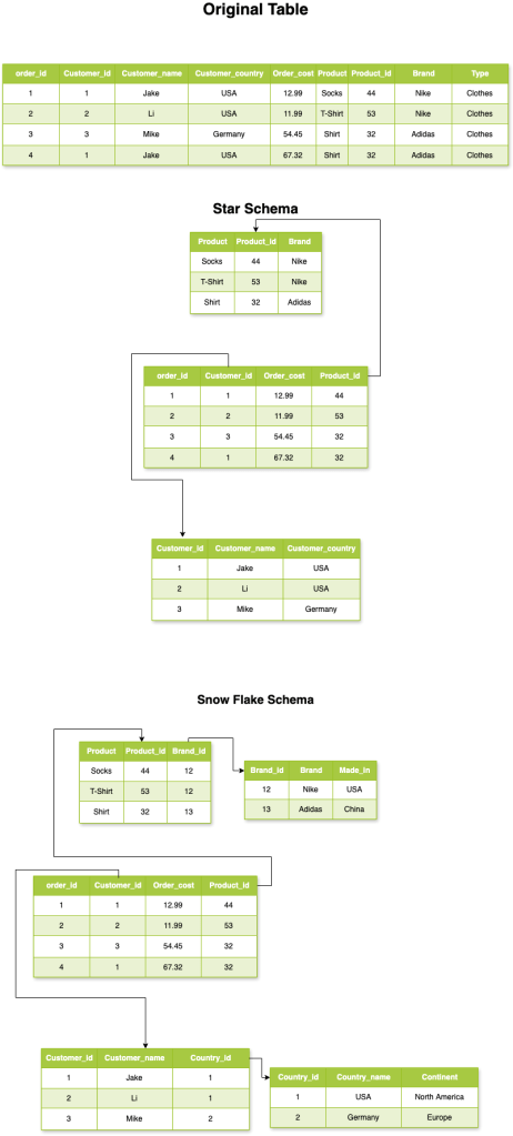
Each has its strengths depending on your use case:

If your priority is query speed and simplicity, go with a Star Schema — fewer joins, faster results.

If you care more about storage efficiency and normalization, a Snowflake Schema is a better fit. It reduces duplication. However, it requires more joins.

Understanding these patterns is key to designing Redshift tables that scale well and perform reliably.

🏗️ Redshift Architecture: How It Really Works

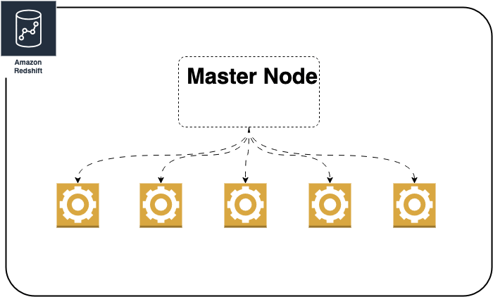
Now let’s dive deeper into how Redshift actually works under the hood.

Redshift uses a Massively Parallel Processing (MPP) architecture. It splits your data and query workload across multiple compute nodes. This makes things fast and scalable. With the newer RA3 instance types, Redshift decouples storage from compute. You can scale your processing power without being limited by how much data you’re storing. This helps keep performance even as your data grows into the terabytes or petabytes.

At a high level, a Redshift cluster consists of a leader node. The leader node plans and coordinates queries. The cluster also has one or more compute nodes. The compute nodes do the actual work.

Now imagine you have a table with billions of orders and another one with millions of product details. How these tables are distributed across the nodes is crucial. Additionally, how Redshift shuffles the data between them during a join can make or break your query performance.

In short: Redshift is fast, but only if you help it be smart about where the data lives.

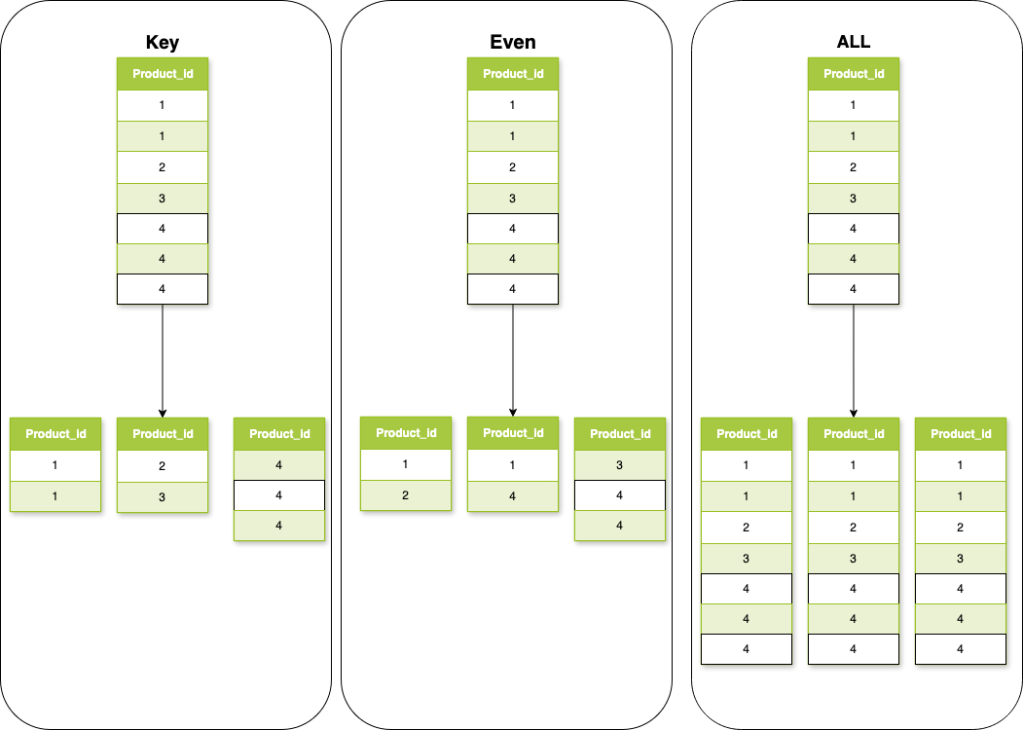
🔄 Redshift Distribution: How Data is Spread Across Nodes

When it comes to how Redshift spreads your data across nodes, there are a few key distribution styles — and choosing the right one can seriously affect performance.

Let’s break down the main types in a simple way:
✅ 1. EVEN Distribution

Imagine you have 10 rows and 5 nodes. With EVEN distribution, Redshift just spreads the rows equally — so each node gets 2 rows, no matter what’s in them.

✔️ Simple

❌ Doesn’t optimize for joins

✅ 2. KEY Distribution

Now let’s say your table has a column called product_id with 6 unique values, and you set your distribution style to KEY on product_id.

Redshift will group all rows with the same product_id on the same node. For example:

Node 1 might handle all rows with product_id = 1

Node 2 gets product_id = 2

Node 3 might get both product_id = 5 and 6

The idea is: each node becomes responsible for specific keys

This helps avoid data reshuffling during joins when the other table also uses the same distribution key.
✅ 3. ALL Distribution

This one is pretty straightforward: Redshift copies the entire table to every node in the cluster.

So if you have a small table — like a product_category or country_lookup table — every node gets a full copy. This means:

✔️ No need for reshuffling when joining — every node already has the data it needs

❌ But if the table is large, this becomes expensive and inefficient (since it’s copied everywhere)

Best for: Small dimension tables that are used in many joins.
✅ 4. AUTO Distribution

If you don’t want to think about distribution styles (yet), just go with AUTO.

Redshift will automatically choose the best distribution style based on the table size and usage patterns. For example:

Small tables may default to ALL

Larger tables may use EVEN

And as your data grows or your usage changes, Redshift might switch strategies under the hood. It’s great for getting started — but keep an eye on it once your data model gets more complex.
✅ 5. NONE or DEFAULT

Technically, not a distribution style — but if you don’t explicitly set a distribution style and you’re on legacy node types (like DC2), Redshift will default to EVEN.

On RA3 with AUTO, you’ll get more flexibility — but if you want full control, it’s always better to explicitly define your distribution.
🧠 Final Thought:

Choosing the right distribution is one of the easiest (and most impactful) ways to avoid slow queries and massive reshuffling. Think about how your tables are joined, and use:

KEY for large fact tables that share join columns

ALL for small dimension tables

EVEN if you just want uniform distribution

AUTO if you’re not ready to decide yet

🎉 Schema? ✅ Distribution? ✅ Now It’s Time to Load Your Data

So, you’ve built your schema, picked the right distribution styles, and your tables are ready to roll. Nice work!

Now comes the fun part — loading your data.

Let’s be honest: most of us start by using INSERT because it feels simple. One row at a time. Job done, right?

But here’s the thing: Redshift is not your everyday transactional database. It’s built for massively parallel processing — and INSERT just doesn’t cut it.

If you’re loading anything more than a few rows, using INSERT is like filling a pool with a coffee mug — slow, inefficient, and frustrating.

---

❌ Why INSERT Falls Apart at Scale

Say you’re inserting thousands (or even millions) of records. With INSERT, each row gets written individually, which means:

• 🐢 It’s slow — especially with larger datasets
• 💥 It eats up more memory and CPU
• 🚫 It doesn’t run in parallel across your Redshift nodes
• 🧨 It’s prone to failure mid-load (especially over a flaky connection)

---

✅ Meet COPY: The Right Way to Load Data into Redshift

Instead of inserting one row at a time, COPY lets you load millions of rows in one shot, using files stored in S3.

Here’s how it looks:

With COPY, you get:

• 🚀 Massive speed — thanks to parallel processing
• 🧠 Smart efficiency — especially with compressed formats like GZIP or Parquet
• 🔁 Bulk loading — designed for data pipelines and ETL jobs
• 🧱 More stability — fewer points of failure

💡 Fun fact: Loading 1 million rows with INSERT can take over an hour. With COPY, you’re done in under a minute.

🚫 Avoid SELECT * — Be Intentional

It might be tempting to just write:

SELECT * FROM orders;

But doing that pulls every single column, even the ones you don’t need — which:

• Increases memory usage
• Slows down query performance
• Makes dashboards and apps slower

✅ Always specify only the columns you actually need:

SELECT order_id, customer_id, total_amount FROM orders;

🔍 Keep Things Fresh with ANALYZE and VACUUM

Just like your house gets messy over time and needs a good cleanup, your Redshift tables need some routine maintenance too — especially after loading, updating, or deleting lots of data.

Let’s break it down:

---

🧠 ANALYZE: Give Redshift a Cheat Sheet

Every time you run a query, Redshift has to figure out the best way to do it — like choosing the fastest route on Google Maps. To do that, it needs up-to-date stats about your data.

That’s where ANALYZE comes in.

It tells Redshift:

“Hey, here’s what the data looks like now — how many rows, how unique each column is, etc.”

With that info, Redshift can:

• Pick the best join methods
• Avoid unnecessary steps
• Run your queries faster

If you skip ANALYZE, Redshift might make bad guesses — which means slow performance.

---

🧹 VACUUM: Rearranging the Furniture (and Taking Out the Trash)

When you delete or update data in Redshift, the old rows don’t get removed right away — they just hang around, taking up space.

VACUUM comes in to:

• Reclaim that wasted space
• Re-sort the data, especially if you’re using sort keys

Why does sorting matter? Because sorted data means Redshift can find what it needs faster — like looking through a tidy bookshelf instead of a messy pile.

---

🧰 When to Use Them

You can run both manually:

ANALYZE;
VACUUM FULL;

Or better yet, bake them into your ETL jobs to run automatically after:

• A big data load
• Lots of deletes or updates

---

🧠 Think of ANALYZE as updating Redshift’s GPS, and VACUUM as a spring-cleaning to keep things running smooth.

Do it regularly, and your queries will thank you. 🙌

🎯 Wrapping Up — and What’s Next

So there you have it — the fundamentals of getting Redshift to work for you, not against you.

From smart schema design and choosing the right distribution style, to loading data efficiently and keeping things tidy with ANALYZE and VACUUM, you’ve now got a solid foundation to build on.

But we’re just getting started.

In the next part of this series, we’ll dive into advanced Redshift optimization techniques — the kind of stuff that makes a real difference when you’re dealing with large-scale data or complex analytics pipelines.

Here’s a sneak peek at what’s coming:

🔧 Sort keys deep dive — how they work, when to use compound vs interleaved
📦 Column encoding strategies — save space, boost speed
🧠 Concurrency scaling and workload management (WLM) — keeping performance stable under pressure
📊 Query tuning 101 — how to debug slow queries with EXPLAIN and system tables
🧰 Materialized views & result caching — smart tricks to save time (and money)
📈 Monitoring tools & dashboards — keeping an eye on performance without drowning in metrics

If that sounds like your kind of thing — stay tuned.
Or better yet, subscribe so you don’t miss the next post! 🚀

Until then, keep building smart.